When the Database Becomes the Bottleneck: A Story of Query Optimization

A walkthrough of problem identification, optimization, benchmarking, and lessons learned

There’s a particular kind of satisfaction in making something slow go fast. Finding the bottleneck, understanding the system deeply, turning sluggish into elegant — I never get tired of it. This is a pattern I’ve seen again and again in software development: everything holds together under normal load, something shifts, and suddenly the cracks appear.

This is the story of one of those moments.

📉 The Day Everything Slowed Down 🐢🐢🐢

It was one of the peak shopping season — the kind of traffic spike every engineering team quietly dreads. Our service, which handles high-frequency transaction lookups, started showing slow response times under the increased load. It was roughly 3x the usual request rate, and the PostgreSQL’s database CPU was hitting its limits — on a database that was otherwise sufficiently sized to handle the anticipated load under normal conditions.

The immediate fix? We scaled up the database reader instance. More CPU, problem resolved, everyone breathed again.

But it nagged at me. We’d run performance tests showing the system should handle far more than what we’d just experienced. So why did it fall over?

Something was off. We just didn’t know where yet.

🤔💭 Asking the Right Questions

Before jumping to conclusions, we asked ourselves the questions:

• Did any unusually heavy background tasks run during that time?
• Had we seen anything like this before?
• Was there a correlation between scheduled cleanup jobs and the load spike?
• Why didn’t performance tests catch this?
• Was there something in the infrastructure causing daily spikes at the same time?

All valid questions. And all, at first, without clear answers.

🕵 Finding the Culprit

The turning point came when we enabled slow query logging on the database. By default, this was off — which means you’re flying blind in production. We set a threshold (around 150ms to start with as the response got super slow) and started watching.

What we found was illuminating: one particular query pattern was showing up repeatedly, with execution times well above our threshold.

The query itself was conceptually straightforward: fetch the most recent transactions for a user, where the user could be identified by any one of three different identifiers, filtered to a specific merchant, ordered by date, with a row limit. Something like:

SELECT <columns>
FROM transactions
WHERE (
    initiated_at >= <year ago>
    AND (
        identifier_a = :value
        OR identifier_b = :value
        OR identifier_c = :value
    )
    AND merchant_id = :merchant
)
ORDER BY initiated_at DESC
LIMIT 2000;

Looks reasonable, right? The problem was what the database was actually doing with it.

🔎 Reading the Query Plan

Using PostgreSQL’s EXPLAIN ANALYZE, we could see exactly what was happening under the hood.

The planner was doing a BitmapAnd across multiple index scans (each column in where had own index) — scanning the index for identifier_a, for identifier_b, for identifier_c, AND for merchant_id separately, then combining the results. The merchant_id condition alone was touching tens of thousands of rows before being filtered down.

This explains why performance tests missed it. The test data distribution didn’t match production — merchants in the real world have wildly different transaction volumes. Some have a handful of records; others have tens of thousands. Our test data was too uniform to expose this edge case.

Here’s a simplified view of the bottleneck:

BitmapAnd
├── BitmapOr (identifier scans — fast, few rows)
│   ├── Index Scan on identifier_a  → ~few rows
│   ├── Index Scan on identifier_b  → ~few rows
│   └── Index Scan on identifier_c  → ~few rows
└── Index Scan on merchant_id       → TENS OF THOUSANDS of rows ← this was the problem

The merchant index scan was doing the heavy lifting, and at peak load with large merchants, it was brutal.

🛠️ The Fix: Composite Indexes

The core insight: instead of scanning merchant_id broadly and then filtering, we should pre-narrow with the user identifier first, then hit merchant and date together — all in one index traversal.

We created three new indexes, one per identifier type, each including merchant and date:

CREATE INDEX idx_transactions_identifier_a_merchant_date
    ON transactions (identifier_a, merchant_id, initiated_at DESC);

CREATE INDEX idx_transactions_identifier_b_merchant_date
    ON transactions (identifier_b, merchant_id, initiated_at DESC);

CREATE INDEX idx_transactions_identifier_c_merchant_date
    ON transactions (identifier_c, merchant_id, initiated_at DESC);

Why composite indexes work here: An index on (a, b, c) can be used for queries filtering on just a, on a + b, or on a + b + c. The leftmost column anchors the traversal. By putting the unique user identifier first, we instantly narrow the search space; merchant_id and initiated_at then serve as an in-index filter and sort, meaning we never need to touch the actual table rows for the ordering step.

A quick note on the trade-off: Adding indexes isn’t free — each new index consumes disk space and adds a small overhead to write operations, since the index must be updated on every insert or update. In a write-heavy system, this deserves careful thought. In our case, the table was roughly 90% reads, so the trade-off was an easy call.

We also explored rewriting the query using UNION — splitting the OR into three separate branches so each could cleanly use its dedicated index. It’s a valid technique and worth knowing. But here’s the thing: we never had to ship it. Once the composite indexes were in place, PostgreSQL’s query planner picked them up automatically and started using them efficiently — no query rewrite needed.

That was a satisfying moment. Sometimes the right move is to give the database the right tools and let it do its job.

📝 What the Query Planner Actually Does

With the right indexes in place, PostgreSQL can internally:

• Use Bitmap Index Scans to combine multiple index conditions
• Perform a Bitmap Heap Scan to fetch only the relevant rows
• Avoid full table scans entirely
• Skip explicit sorting when the index already provides order

Here’s a simplified view of the shift, before and after:

Before:
  Seq Scan → Filter → Sort → Limit

After:
  Bitmap Index Scan → Bitmap Heap Scan → Limit
  (or)
  Index Scan → (Already Sorted) → Limit

And a simplified EXPLAIN output after the new indexes:

Bitmap Heap Scan on transactions
  Recheck Cond: (identifier_a = ? OR identifier_b = ? OR identifier_c = ?)
  -> BitmapOr
       -> Bitmap Index Scan on idx_transactions_identifier_a_merchant_date
       -> Bitmap Index Scan on idx_transactions_identifier_b_merchant_date
       -> Bitmap Index Scan on idx_transactions_identifier_c_merchant_date

Notice what’s happening: the database is combining multiple index paths intelligently. It is not blindly scanning the table. The original query, unchanged, now runs in single-digit milliseconds instead of 150–200ms during the peak.

Don’t fight the database — enable it.

Before: Execution time ~150–200ms, dominated by a broad merchant scan.
After: Execution time in single-digit milliseconds always.

📐 Benchmarking It Properly

A few things worth knowing about benchmarking PostgreSQL queries:

• EXPLAIN alone doesn’t run the query — it estimates. Use EXPLAIN ANALYZE for real numbers.
• Run the same query multiple times and average the results. Disk cache effects can skew a single run.
• Client overhead is real — measure execution time from the planner output, not just what your application sees.
• Tools like DataGrip can visualize the query plan graphically, which makes it much easier to spot where the time is being spent.

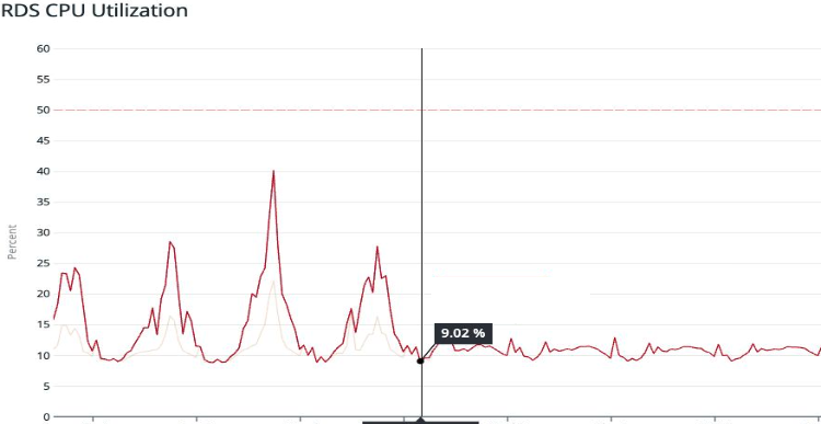
We validated in a staging environment first, checked that DB CPU load dropped significantly under the same simulated load, and then rolled out to production.

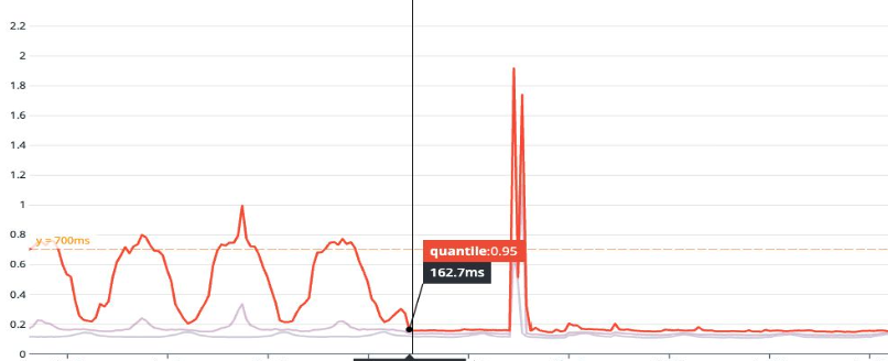
The results in production confirmed it: CPU utilization dropped substantially. Application-level latency at the 99th percentile improved dramatically. The query that had been dominating our Top SQL list vanished from the charts.

API response time

🤔 Why Didn’t the Performance Tests Catch This?

This one still stings a little, but it’s an honest lesson.

Our performance test data was generated with relatively uniform distributions across the dimensions that matter here — specifically, merchant transaction volumes. In production, some merchants have orders of magnitude more transactions than others. The tail of that distribution is where the slow query lives.

The gap: Test input data that doesn’t reflect real production data distribution will miss these kinds of volume-sensitive performance cliffs.

It’s genuinely hard to get right. You’d need to either sample real data shapes or build test data generation that deliberately includes high-cardinality edge cases.

💡 Lessons Learned

These are the takeaways to carry forward:

Enable slow query logging in production. Not just temporarily — keep it on at some reasonable threshold. You want visibility before an incident happens, not during one.

The OR problem is real, but indexes can solve it without query rewrites. An OR across indexed columns forces the planner to merge multiple index scans. With the right composite indexes, the planner can still use them efficiently via BitmapOr — and you may not need to touch the query at all.

Composite indexes are powerful when designed around your query patterns. Think about the column order: high-selectivity (unique or near-unique) columns first, then filters, then sort keys. A well-designed composite index can cover the full query without touching the heap.

Performance tests need realistic data. Distribution matters more than volume. E.g. 50M uniformly distributed rows can behave completely differently from 50M rows with realistic skew.

Production is its own environment. Some issues only emerge at real scale, with real data shapes, under real load patterns 😅. That’s not a failure — it’s just the nature of complex systems.

Trust the query planner — and give it what it needs. PostgreSQL’s planner is sophisticated. Once the right indexes exist, it often makes the right choices on its own. Before rewriting queries, ask whether the planner just needs better indexes to work with. When one query was consuming a large share of DB CPU, everything else suffered. Fix the bottleneck, and the whole system breathes easier.

📌 A Note on Patience

Reading query plans is a skill that takes time to develop — to understanding how statistics, cost estimates, and index structures interact. But that’s also what makes it rewarding. Each slow query is a small puzzle, and when the execution time drops from hundreds of milliseconds to a handful, it feels genuinely good.

If you’re debugging similar issues, EXPLAIN ANALYZE, composite index design, and PostgreSQL’s documentation on query costs are great places to start. Understanding what the planner is actually optimizing for will change how you write queries.

Useful resources

PostgreSQL Analyze queries and PostgreSQL® EXPLAIN – What are the Query Costs?
How To Benchmark PostgreSQL Queries Well
Avoiding “OR” for better query performance
Index Creation in PostgreSQL Large Tables: Checklist for Developers